mpiprofile

Overview

Teaching: 20 min
Exercises: 20 min

Questions

• How to improve the performance of MATLAB code?

• What is profiling?

• How to profile your code in MATLAB?

Objectives

• To learn to profile MATLAB code using MATLAB’s profiler.

Profiling the parallel code - mpiprofile

Profiling parallel code in MATLAB is similar to profiling serial code. For profiling parallel code, we have to use the mpiprofile command. The difference between using the standard profile and mpiprofile commands is in where they are called.

Similar to the serial profiler, mpiprofile can be used from either the command prompt (pmode) or within the MATLAB script. For interactive usage, mpiprofile should be called from the parallel command window (pmode).

Open the pmode and enter the following commands at the pmode command prompt.

P>> mpiprofile on
P>> distobj = codistributor('1d',1);
P>> A = rand(10, distobj);
P>> B = A*A;
P>> mpiprofile viewer

Once we execute mpiprofile viewer command in the pmode, it will open a new window with the profiling data. Clearly, the Profiler window for mpiprofile contains many more columns when compared with the serial profiler. This is to be expected because a parallel job involves data communication among workers. Therefore, it is very important to know the amount of data communicated from one worker to the other, along with the time spent in communicating the data.

The profile summary contains nine columns:

• Column 1: Function name
• Column 2: Calls - Number of times the function was called on this worker
• Column 3: Total Time - The total amount of time this worker spent executing this function
• Column 4: Self Time - The time this worker spent inside this function, not within children or local functions
• Column 5: Total Comm Time - The total time this worker spent transferring data with other workers, including waiting time to receive data
• Column 6: Self Comm Waiting Time - The time this worker spent during this function waiting to receive data from other workers
• Column 7: Total Interlab Data - The amount of data transferred to and from this worker for this function
• Column 8: Computation Time Ratio - The ratio of time spent in computation for this function vs. total time (which includes communication time) for this function
• Column 9: Total Time Plot - Bar graph showing the relative size of Self Time, Self Comm Waiting Time, and Total Time for this function on this worker

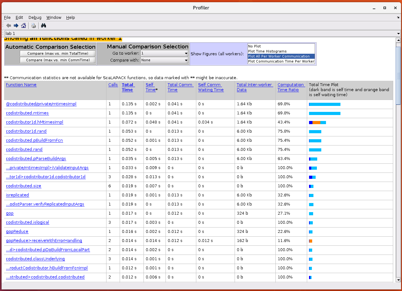
The default window displays the data in a tabular form. We can visualise the communication details by selecting from the options in the Show Figures (all workers) section. By choosing these options, we can get the information on communication.

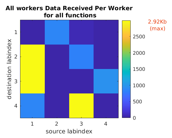
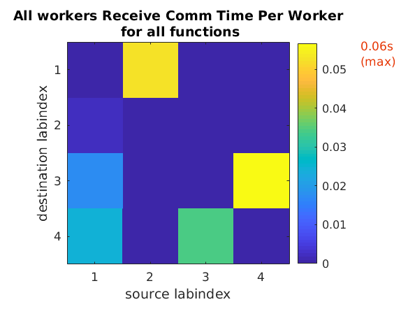
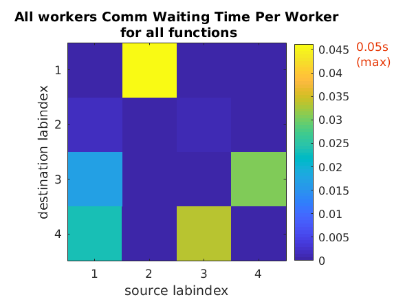
You can run mpiprofile and observe if there are any noticeable differences in the amount of data communicated and the communication time by replacing codistributor('1d',1) with codistributor('1d',2) and codistributor('2dbc').

P>> mpiprofile on
P>> distobj = codistributor('1d',2);
P>> A = rand(10, distobj);
P>> B = A*A;
P>> mpiprofile viewer

P>> mpiprofile on
P>> distobj = codistributor('2dbc');
P>> A = rand(10, distobj);
P>> B = A*A;
P>> mpiprofile viewer

Exercise - Profiling parallel direct solver

In this exercise, we use the code for parallel direct solver from the spmd lesson to gain further understanding of mpiprofile.

Use following code to see which parts of the code are expensive, and then think of solutions for improving the performance.

P>> mpiprofile on
P>> n = 1000;
P>> distobj = codistributor1d();
P>> ADist = rand(1000, distobj);
P>> bDist = sum(ADist,2);
P>> xDistEx = ones(n,1,distobj);
P>> xDist = ADist\bDist;
P>> errDist = norm(xDistEx-xDist)
P>> mpiprofile viewer

mpiprofile outside the pmode

If we want to obtain the profiling data for a communicating job when running outside the pmode, for example, with scripts, then it’s much more involved.

We have to modify user functions to return output arguments of mpiprofile info using its functional form. For example,

function [pInfo,yourResults] = myfunc1
    mpiprofile on

    myData = rand(100, codistributor()) );

    pInfo = mpiprofile('info');

    yourResults = gather(myData,1);
end

Unfortunately, there is not much information on this topic expect what is available at mpiprofile example. We will update this material if we come across any good examples.

Key Points

• Always profile your code before working on optimisations for performance.

• Use a minimalistic data set while profiling your code.

• Understanding communication pattern is key to understanding parallelisation.

• Check communication and waiting times of each participating worker to identify potential bottlenecks and critical paths.